Work / JWST pipeline
From raw detector reads to a calibrated JWST image
JWST's detectors record how charge builds up in every pixel. The calibration pipeline turns those raw ramps into images and spectra a scientist can trust. I worked with the official pipeline and the MIRAGE simulator, and this page follows the detector-level stage, where most of the instrument's quirks get cleaned up.
Research project at IIT Hyderabad, under the guidance of Prof. Mayukh Pahari.
Four stages
Goes in
Raw spacecraft telemetry.
What happens
The Science Data Processing system turns the telemetry into FITS files and fills in the metadata: observation details and spacecraft information.
Comes out
Uncalibrated files named *_uncal.fits. Each is a four-dimensional array of pixel values across integrations and groups, and the starting point for offline processing.
Goes in
The *_uncal.fits files: each pixel's ramp of non-destructive reads.
What happens
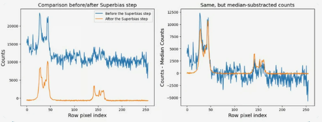
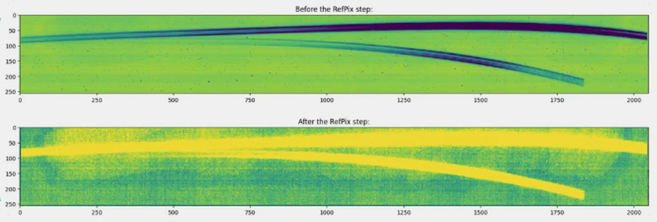
Detector effects are corrected one step at a time: data-quality flags, saturation, superbias, reference pixels, linearity and dark current, then jump detection and ramp fitting.
Comes out
A count-rate image in counts per second for each exposure, *_rate.fits. This is the stage my plots below come from.
Goes in
The count-rate images from Stage 1.
What happens
Sky coordinates are attached (and wavelengths, for spectra), pixel-to-pixel sensitivity is corrected with a flat field, and counts are converted into physical flux units.
Comes out
Calibrated single exposures, *_cal.fits.
Goes in
Calibrated exposures of the same target.
What happens
Exposures are combined, outliers such as leftover cosmic rays are rejected, and everything is resampled onto a common grid. Then the science products are extracted: photometry, source catalogues and spectra.
Comes out
Combined images, catalogues and one-dimensional spectra, ready for analysis.
Up the ramp
A detector never takes a single picture. It reads each pixel again and again while charge builds up, and the slope of that ramp is the count rate, the number the pipeline wants. A cosmic ray adds a sudden jump, and a straight line fitted through the jumped ramp gives the wrong rate. Stage 1 flags the jump and fits the pieces either side.
What the steps do to real data
To see the corrections at work, I ran exposures through Stage 1 and plotted the result before and after individual steps. These are from my own runs.